Calculation And Interpretation

The Arithmetic Mean is the simplest and the most popular parameter characterizing a center of values’ dispersion.  As such it is also used to estimate the Expected Value.  It is calculated as follows:

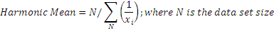
The Harmonic Mean is used in frequency data analysis or to compute the general mean value based on the means of data subsets. It is also the preferable method for averaging ratios like Price/Earnings as the harmonic mean is especially sensitive to small values. The harmonic mean is computed as:

The Geometric Mean is applied when dealing with percentages and rates of change; it is computed as:

Of the three means discussed, the arithmetic mean always yields the highest result, while the harmonic mean yields the lowest.

The Quadratic Mean, also called Root Mean Square (RMS), is used in situations where the square of the values matters; particularly, it is useful as a measure of the amplitude of randomly varying quantities and as a measure of some performance parameters. The calculation is:

The Median is determined by sorting the data set in ascending order and picking the point in the middle of the sequence so that number of points above and below the median is the same.  When the number of data points is even, the Median is computed as the average of the two middle values.  Unlike the Mean, the Median is not influenced by outliers at the extremes of the data set and hence the Median and the mean together give a better view of the spread of the numbers.

The Midrange is the point halfway between the two extremes (see also about the Range):

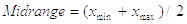
As an indicator of the central tendency of the data it is not robust for small data sets.

The RawMoment (i.e. moment about zero) is the Expected Value over the data set:

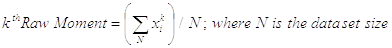
So the First Raw Moment is the Arithmetic Mean of data set values, the Second Raw Moment is the Arithmetic Mean of squared values and so on.

As a rule, highest Raw Moments are used in user-specific cases.

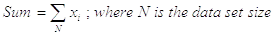
The Sum is a result of addition over all data points available:

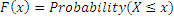
The Cumulative Distribution function (CDF, usually denoted as F(x)) represents the probability that the random variable X takes on a value less than or equal to x:

The probability that X lies in the interval (a, b] is:

The Quantile function of a distribution is a number x such that a given proportion (probability) p of the data set values are less than or equal to x; that is, it returns the greatest value of x such that:

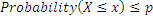
The function is defined for real p between zero and one and is mathematically the inverse of the cumulative distribution function.

Users usually need to know key percentage points of a given distribution and most usable Quantiles have special names:

• The 4-Quantiles where p takes 0.25, 05, 0.75 or 1 are called Quartiles
• The 10-Quantiles where p takes from 0.1, 0.2, … 0.9, 1  are called Deciles
• The 100-Quantiles are called Percentiles

The Order Statistic of a data set is equal to its smallest value. So the Min of the data set has index zero and the Max is the order statistic.

Min and Max present respectively the minimum and the maximum of data set values also called the largest observation and smallest observation.

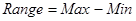
The Range is amplitude excursion which serves as the simplest measure of dispersion:

The Variance and the Standard Deviation are commonly used as such to measure dispersion and also to compute other statistics.

The variance is calculated by taking the arithmetic mean of the squared differences between each value and the mean value:

Squaring makes each term positive and adds more weighting to bigger differences.

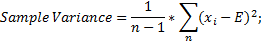
To get an unbiased estimation of the variance value when dealing with samples, the modified calculation is applied:

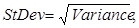
The Standard Deviation is the square root of the variance and has the same units of measure as the variable processed:

Be careful between the distinction of the population and sample variances (or standard deviations), as they have different definitions. You have to realize the difference between a sample and the population it was drawn from. There are separate properties to distinguish the population and sample variances. Variance property and VariancePopulation property are identical.

For standard deviations there are also separate properties StandardDeviation, StandardDeviationPopulation and StandardDeviationSample, again StandardDeviation and StandardDeviationPopulation are identical.

The Coefficient of Variation (also known as Unitized Risk or the Variation Coefficient) allows measuring dispersion relative to the Expected Value.  It is a useful statistic for comparing the degree of variation from one data series to another, even if the means are significantly different from each other.

In mathematical sense, it is defined as the standard deviation normalized by the mean, i.e. as the ratio of the standard deviation to the arithmetic mean:

The ratio is evidently defined for non-zero mean and is most useful for variables that are always positive.

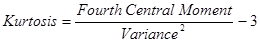
The Kurtosis (also known as Excess Kurtosis) is a measure of whether the data are peaked or flat relative to normal distribution and this way characterizes the shape of a distribution: the kurtosis of the normal distribution is zero by definition; if the kurtosis is negative then the distribution is flatter (observations are spread in a wider fashion) than normal and vice versa.  Its value does not depend on an arbitrary change of the scale and location of the distribution.

The kurtosis is computed as:

The Skewness measures deviation of a distribution from symmetry around the mean so that the value near to zero points out perfect symmetry when the mean and the median are almost equal; negative values for the skewness indicate data that are skewed left so the mean is less than the median and vice versa.

The skewness is calculated as:

The Central Moment (i.e. moment about the Expected Value) is computed as:

So the First Central Moment is zero by definition, the Second Central Moment presents the variance.

Highest Central Moments are commonly used as components for other and user-defined statistics.