Nonlinear Least Squares (NLS) Problem

The problem is formulated in the form:

Given an m-component vector y of real-world observations, should find the best approximation of the observations with some user-defined nonlinear model function m(x) of n arguments in the sense that the sum of squared residuals is the minimum:

min _x || f(x) ||² = min _x || y - m(x) ||² ,

where:

• x is n-component vector of unknown parameters, m ≥ n;

• f(x) denotes the objective function: f(x) = y - m(x);

• || ... || stands for Euclidean norm.

Usually, there is no closed-form solution to a NLS problem. Instead, iterative numerical algorithms are used to find the optimum.

The NonlinearLS class is destined to solve the unconstrained NLS problem. The class realizes Trust Region optimization strategy with the parameters described below.

To initialize a class instance instance use one of the two constructors provided, both of them require a delegate method to implement the objective function:

• NonlinearLS(Int32, Int32, NonlinearLSFunctionDelegate, NonlinearLSGradientDelegate)

• NonlinearLS(Int32, Int32, NonlinearLSFunctionDelegate)

The NLS solver is controlled by stopping criteria that have default values assigned while class initialization and should be customized (if necessary) before running of optimization process; the default values are the recommended ones and suitable in most practical applications. The stopping criteria are available for modification as class properties:

Index	Property	Default Value	Restriction	Description
0	TrustRegionAreaBound	1E-6	1E-6 .. 0.1	The upper bound for Trust Region Radius: the current Radius value below this limit indicates that the process has converged.
1	ResidualTolerance	1E-6	1E-6 .. 0.1	The tolerance for Euclidean norm of residuals: Objective function below this limit indicates that the required precision is gained.
2	JacobiMatrixTolerance	1E-6	1E-6 .. 0.1	The tolerance value for determining that Jacobi matrix is singular: The norm of the Jacobian below this limit indicates that the process can not be continued.
3	TrialStepTolerance	1E-6	1E-6 .. 0.1	The tolerance for step length: The current value of the trial step length below this limit indicates that the process has converged.
4	ResidualDecreaseTolerance	1E-6	1E-6 .. 0.1	The tolerance (lower bound) for objective function (residual) decrease. Regulates dynamic of convergence: the process is stopped when regular iteration results in lower decrease of the objective function than this limit.
5	TrialStepPrecision	1E-10	1E-10 .. 0.1	Trial step precision: Defines required accuracy when solving of subprobem (precision of approximation of the objective function in the Trust Region area).
N/A	JacobiMatrixPrecision	1E-5	1E-5 .. 0.1	The precision of the Jacobi matrix calculation: used for numerical approximation of the Jacobian and stops calculations when Jacobian norm becomes lass than this limit.
N/A	TrialStepIterationLimit	100	> 1	The maximal number of trial steps (global iterations).
N/A	TrustRegionIterationLimit	1000	> 1	The maximal number of iterations on each trial step to solve the subproblem .
N/A	InitialStepBound	100.0	0.01 .. 100.0	Initial trial step length.  Note Does not serve as stopping criterion.

Any of trial step related criteria can terminate optimization process; for diagnostic reason the most important criteria are indexed.

Optimization process is started with one of the two methods, either with user-specific or default start point with all zero components:

• Minimize(Vector)

• Minimize

The results of optimization are reflected by the corresponding properties:

The sample below demonstrates using of the NonlinearLS class to solve the following problem:

Given five observations of the dependent variable as a vector y = [ y_i ], i = 1 .. 5, and the corresponding observations of three independent variables as a matrix A whith rows corresponding to observations and columns to variables, should approximate the observations y with the two-parameters nonlinear model function:

In this problem, the objective function is:

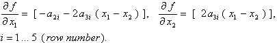
This function is differentiable so the Jacobian can be expressed analytically. The gradients (columns of the Jacobian) are as follows:

The code snippet uses the class with the methods-delegates named Function and Jacobian:

 1using System;
 2using FinMath.LinearAlgebra;
 3using FinMath.NumericalOptimization.Unconstrained;
 4
 5namespace FinMath.Samples
 6{
 7    public class NonLinearLeastSquares
 8    {
 9        static readonly Matrix A = Matrix.Random(10, 3);
10        static readonly Vector Y = Vector.Random(10);
11
12        static void Main()
13        {
14            // Initialize the NLS solver with the delegate methods defined just below.
15            NonlinearLS nls = new NonlinearLS(2, A.Rows, Function, Jacobian);
16
17            // Run the optimization.
18            if (nls.Minimize())
19            {
20                // Optimal solution.
21                Console.WriteLine($"MinimumPoint = {nls.MinimumPoint.ToString("0.000")}");
22
23                // What criterion triggered.
24                Console.WriteLine($"Criterion Index = {nls.StopCriterion}");
25
26                // The number of iterations.
27                Console.WriteLine($"Iterations done = {nls.IterationsDone}");
28
29                // Resulting decreasing of the objective function.
30                Console.WriteLine($"Optimization Gain = {(nls.InitialResidual - nls.FinalResidual):0.000}");
31            }
32            else
33            {
34                Console.WriteLine("Optimization failed.");
35            }
36        }
37
38        static void Function(Vector x, Vector f)
39        {
40            for (Int32 i = 0; i < A.Rows; i += 1)
41            {
42                f[i] = Y[i] - A[i, 0] - A[i, 1] * x[0] - A[i, 2] * Math.Pow(x[0] - x[1], 2.0);
43            }
44        }
45
46        public static void Jacobian(Vector x, Matrix g)
47        {
48            for (Int32 i = 0; i < A.Rows; i += 1)
49            {
50                g[i, 0] = -A[i, 1] - 2 * A[i, 2] * (x[0] - x[1]);
51                g[i, 1] = 2 * A[i, 2] * (x[0] - x[1]);
52            }
53        }
54    }
55}

Reference

Other Resources