Monte Carlo Model |
Monte Carlo method is particularly useful in the valuation of options with multiple sources of uncertainty or with complicated features which would make them difficult to value through a straightforward Black-Scholes-style or lattice based computation. The technique is thus widely used in valuing path dependent structures like lookback- and Asian options and in real options analysis.
The technique applied is:
to generate several hundred thousand possible (but random) price paths for the underlying via simulation
to calculate the associated exercise value (i.e. "payout") of the option for each path
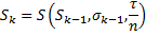
to approximate the expected continuation payoffs at each time step and compare their discounted values with the immediate exercise values. In case the exercise payout at the step is greater, set it to immediate exercise value.
the exercise payouts at the actual exercise decision step are then averaged and discounted to today. This result is the value of the option.
Hereinafter the following notation is used:
S, be the price of the stock.
K, the strike of the option.
r, the risk-free interest rate.
q, the annual dividend yield.
μ, the drift rate of S, annualized.
σ, the volatility of the stock's returns.
τ, the time to expiry of the option.
n, the number of steps.
m, the number of paths generated.
l, the number of basis functions to use in approximation of expected continuation payoff.
This topic contains the following sections:
Monte Carlo model assumes one of the following price models:
risk neutral geometric Brownian
geometric Brownian
other (user specified)
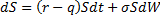
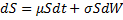
The price of the underlying instrument S is usually modeled such that it follows a geometric Brownian motion with constant drift μ and volatility σ. dW is found via a random sampling from a normal distribution. In a risk neutral model μ = r-q.
The underlying stock price is usually assumed to follow a path that is a function of a Brownian motion or a custom user specified function.
To sample a path following this distribution from time 0 to τ, we chop the time interval into n units of length τ/n, and approximate the Brownian motion or calculate the custom function over the interval τ/n.
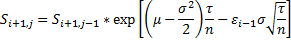
In case of Brownian motion the approximation is made by a single normal variable of mean 0 and variance τ/n. The price for a path i = 0..m and time step j = 1..n is found via the following formula:
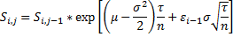
where εi is a draw from a standard normal distribution.
To improve the accuracy the antithetic variates method is used which reduces the variance of the sample paths. Due to the antithetic variates method the above formula is applied to the even paths. For the uneven i the following formula is applied:
In case of a custom price function the paths are generated according to the formula:
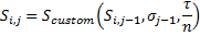
where 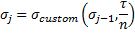 is the custom volatility on a particular time step.
The next step is computing the exercise payouts on each step j for each path i.
European option:
For call:
For put:
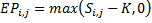
American option:
For call:
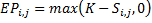
For put:
Custom option:

In case of an option that can be executed at a time step before the expiration we have to approximate continuation (non-execution) payoffs. Continuation payoff are computed at each time step, discounted and compared with the execution payout to make a decision whether to execute an option at the particular step or not.
This estimation is done by stepping backward in time. The continuation payoff can be obtained from the simulated path prices via regression. The fitted value from this regression provides a direct estimate of the expected payoff for each exercise time. Comparing it with the value for immediate exercise, the optimal exercise strategy along each path can be estimated well. Discounting back and averaging these values for all paths results in the present value of the option.
This process shall look as follows:
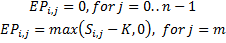
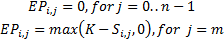
Initialize value for each path as the execution payout at the last step:

Start iterating backwards for each time step j= n-1..0 :
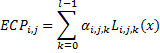
Create a matrix of regression independent variables using the user specified number of basis Laguerre polynomials:


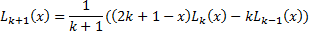
and set x=stock price at the node. Only those points which have a positive immediate exercise value are picked. Rest of the nodes with 0 or negative payoff are ignored for regression input.
Perform Ordinary Least squares to get coefficients αk of basis functions.
Compute expected continuation payoff for each path i:
Compare discounted continuation values with the immediate exercise values. If
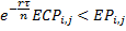 , choose to exercise and assign the value for this path
equal to the exercise value for the current step:
, choose to exercise and assign the value for this path
equal to the exercise value for the current step:

Discount value at each path:

Go to the previous time step until the iterations are done.
Calculate expected payoff by averaging. This gives the option value:

Delegates imply the custom functions computing the price, volatility and exercise payout on each time step. Price and volatility delegates are applied in case of pricing model other than geometric Brownian. Exercise payout delegate is applied in case of custom option type.
Delegate | Description | Performance |
|---|---|---|
custom pricing | Delegate type for sampling asset price change during timeStep time. | |
custom volatility | Delegate type for sampling asset volatility in timeStep time. | |
custom exercise payout | Delegate type for calculating payout of option in case of exercise after timeToMaturity*continuations/steps time. |

The following constructors create an instance of MonteCarlo class with or without usage of performance acceleration.
Constructor | Description | Performance |
|---|---|---|
no acceleration | Constructor without parameters for accelerator usage. | |
use acceleration | Constructor that defines which Greeks should be saved for fast recomputation. Note that at each query for any of saveable Greeks all of them will be computed if needed. The parameters passed in to the constructor are: flag of option value saving and maximum number of data sets allowed to be memorized. |

The following methods initialize the object, set the custom functions and settings and recompute option value.
Method | Description | Performance |
|---|---|---|
initialize | Initializes object by option parameters: stock price, strike price, risk free rate, annual dividend yield, time to maturity, option type, option style, steps, volatility.
| |
set acceleration memory use | Changes acceleration RAM usage. It is a resource-consuming operation which refreshes the accelerator state. | |
set custom price model functions | Sets custom price model functions. This functions are used if and only if price model is PriceModel.Other .
| |
set custom exercise payout | Sets custom option payout function. This function is used if and only if option style is OptionStyle.Other . | |
set custom expected return | Sets custom expected return for geometric Brownian price model. | |
recompute | Forces to compute value of option using new prices paths. |
The class has the following properties that are used to update the source data of the option:
Property | Description | Performance |
|---|---|---|
steps | Number of time steps. | |
price paths | Number of price paths. | |
basis functions | Number of basis functions for least square approximation. | |
exercise payout function | Exercise payout function for custom option style. | |
price model | Price model for custom option style. | |
expected return | Expected return of the underlying asset. Used for geometric Brownian price model. | |
next price | Next price function. Used for custom price model. | |
next volatility | Next volatility function. Used for custom price model. | |
random generator | Random generator used for prices paths generation. |

Monte Carlo valuation example:
 1using System;
 2using FinMath.Derivatives;
 3using FinMath.Statistics.Distributions;
 4
 5namespace FinMath.Samples
 6{
 7    class MonteCarloSample
 8    {
 9        static Normal normal = new Normal();
10        static Double riskFreeRate = 0.009;
11
12        static void Main()
13        {
14            Double stockPrice = 350;
15            Double strikePrice = 370;
16            Double annualDividendYield = 0.05;
17            Double timeToMaturity = 1.06;
18            Int32 numberOfSteps = 200;
19            Int32 numberOfPaths = 10000;
20            Int32 numberOfBasisFunctions = 4;
21            Double volatility = 0.22;
22
23            // Initialize MonteCarlo.
24            MonteCarlo monteCarlo = new MonteCarlo();
25            monteCarlo.InitByVolatility(stockPrice, strikePrice, riskFreeRate, annualDividendYield,
26                timeToMaturity, OptionType.Put, OptionStyle.American, numberOfSteps, volatility);
27            monteCarlo.PriceModel = PriceModel.Other;
28            monteCarlo.PricePaths = numberOfPaths;
29            monteCarlo.BasisFunctions = numberOfBasisFunctions;
30            monteCarlo.SetCustomPriceModelFunctions(NextPrice, NextVolatility);
31
32            Console.WriteLine($"Option value = {monteCarlo.Value:0.000}");
33
34            Double stockPrice2 = 352;
35            Double timeToMaturity2 = 1.05;
36
37            // Update asset stock price and time to maturity.
38            monteCarlo.Update(stockPrice2, timeToMaturity2);
39
40            Console.WriteLine($"Option value = {monteCarlo.Value:0.000}");
41
42            // Use another paths of underlying asset price.
43            monteCarlo.RecomputeValue();
44
45            Console.WriteLine($"Option value = {monteCarlo.Value:0.000}");
46        }
47
48        // Custom price model functions.
49        public static Double NextPrice(Double currentPrice, Double currentVolatility, Double timeStep)
50        {
51            return currentPrice * Math.Exp((riskFreeRate - currentVolatility * currentVolatility / 2) * timeStep +
52                currentVolatility * normal.Sample() * Math.Sqrt(timeStep));
53        }
54
55        public static Double NextVolatility(Double currentVolatility, Double timeStep)
56        {
57            return currentVolatility * Math.Exp(normal.Sample() * timeStep);
58        }
59    }
60}