Basics of Linear Least Squares |
This topic contains the following sections:
- Canonical Linear Least Squares Problem
- Solution
- Computational Details
- Extensions
- Recommendations
- See Also
A variety of LS algorithms is based on the idea developed by Gauss and known as Canonical (or Ordinal) LS form.
This idea gets statistical foundation being derived from the method of moments which is a very general principle of estimation.
The Gauss-Markov theorem states the LS method to be the best linear unbiased estimator of any linear function under the following assumptions:
The residuals are uncorrelated and all have zero means (mean independence);
The residuals have the same variance (homoskedasticity);
The residuals are uncorrelated.
Years of experience have shown that LS produces useful results even if the probabilistic assumptions are not satisfied. Thereupon, the LS principle is mostly known with regard to statistic and especially to regression models which form the core of the discipline of econometrics.
The canonical specification is formulated in context of Regression Analysis.
Given a vector of n observations of the dependent variable (or regressand) y,
and the corresponding n observations of m independent variables (or regressors) x j , j = 1 ... m,
should produce Regression Model of the variables x j on the variable y by a linear combination:

such that
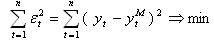 with
respect to the model coefficients
β j ,
with
respect to the model coefficients
β j ,
where:
the subscript t stands for a particular observation number, t = 1 ... n;
the superscript M denotes a model (predicted) value;
ε t is a model residual, the residuals are assumed to be uncorrelated and have zero mean.
The regression coefficients represent contributions of the corresponding regressors to the prediction of the regressand and, this way, reflect statistical partial correlations between the regressors and the dependent variable over the observations (i.e. correlation between the given regressor and the dependent variable when all other predictors are held fixed).
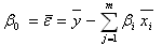
The model intercept, β 0 , binds the mean values of the dependent and independent variables over the observations presenting the average value of the residuals:
In matrix notation the regression model takes the form:
y = X b + e
where:
X is the n-by-m+1 matrix of regressors' observations known as the Design Matrix, the first column of the matrix corresponds to the intercept member and contains all ones;
b is the m+1-component vector of the coefficients to be found, the first element corresponds to the intercept member;
e is the n-component vector of the residuals.
This notation is given with regard to regression with the intercept member. Regression without intercept operates with n-by-m Design Matrix X and m-component vector B. |
Technically, the Least Squares estimator is found by setting to zero the gradient of the sum of squares with respect to betas what results in m Normal Equations:
X TX b = X Ty.
The theoretical closed-form solution of the Normal Equations yields the vector of the optimal coefficients:
b = (X TX)-1X Ty.
There are several difficulties with the theoretical approach as the normal equations are always more badly conditioned than the original overdetermined system, and with finite-precision computation the normal equations can actually become singular, even though the columns of X are independent.
Computational techniques for linear LS problems make use of orthogonal matrix factorizations; the solution based on Singular Value Decomposition (SVD) of the Design Matrix provides robust results even in the case of singularity.
In linear Least Squares, linearity is meant with respect to parameters β j so the extended form of the model can be written as:

where f j ( x j ) are known functions that may be nonlinear with respect to the variable x and used in place of x itself.
The most usable functions are:
Hyperbolic
Exponential
Parabolic
Logarithmic
To provide stability of the estimates with the linear Least Squares, common recommendation is that one should have at least 10 to 20 times as many observations as one has variables.