Augmented Dickey-Fuller (ADF) Test

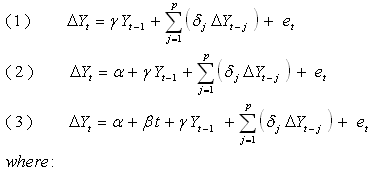
Given an observed time series Dickey and Fuller consider three differential-form autoregressive equations to detect the presence of a unit root:

• t is the time index,

• α is an intercept constant called a drift,

• β is the coefficient on a time trend,

• γ is the coefficient presenting process root, i.e. the focus of testing,

• p is the lag order of the first-differences autoregressive process,

• e_t is an independent identically distributes residual term.

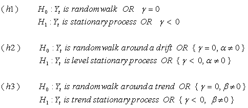
The focus of testing is whether the coefficient γ equals to zero, what means that the original process has a unit root; hence, the null hypothesis of γ = 0 (random walk process) is tested against the alternative hypothesis γ < 0 of stationarity. More detailed, the null and alternative hypotheses corresponding to the models above are:

The ADF test ensures that the null hypothesis is accepted unless there is strong evidence against it to reject in favor of the alternate stationarity hypothesis.

ADF testing technique involves Ordinary Least Squares (OLS) method to find the coefficients of the model chosen. To estimate the significance of the coefficients in focus, the modified T (Student)-statistic (known as Dickey-Fuller statistic) is computed and compared with the relevant critical value: if the test statistic is less than the critical value then the null hypothesis is rejected. Each version of the test has its own critical value which depends on the size of the sample.

There are some drawbacks of the ADF test that require additional efforts to get reliable results.

1. The ADF Test has low statistical power in distinguishing between true unit root processes (γ = 0) and near unit root processes (γ is close to zero). Also, several authors have shown that the ADF test tends to reject the non-stationarity hypothesis far too often, when the series have large (long-run) moving average processes. If there is evidence or doubt about such cases then it is recommended to additionally apply other stationarity tests (for instance, the KPSS Test) to ensure the results.

2. Uncertainty about lags order, p, which has to be determined when applying the test. As it is shown by Perron (1989), including extra regressors of lagged first-differences does not affect the size of the test (probability of Type I Error) but decreases test power. On the contrary, too few lags may affect the size of the test. Perron suggested a procedure to define the adequate lag order. An alternative approach is to examine information criteria (such as the Bayesian, Hannan-Quinn, etc.) computed for different lags.

3. Uncertainty about what test version to use, i.e. about including the intercept and time trend terms. Inappropriate exclusion or inclusion of these terms substantially affects test reliability. Using of prior knowledge (for instance, as result of visual inspection of a given time series) about whether the intercept and time trend should be included is the mostly recommended (but not always possible) informal way to overcome the difficulty mentioned. The more formal (algorithmic) approach is known as testing strategy and requires several additional experiments (series of ordered tests) to decide what model is adequate for a given observed process. There are several testing strategies developed, the most known of them are those suggested by Dolado et al. (1990), by Elder and Kennedy (2001) and by Enders (2004).

The ADFTest class implements ADF Test procedure according to the specification above. This class inherits from the OneSampleTest class.

The following constructor creates an instance of the ADFTest class.

The following public properties provide the details about the model and decision made:

Note
There is also the indicator-style implementation of the ADF Test available in the Financial Analysis library and referred to as C# Copy 1QuantOffice.FinancialAnalysis.TA.AdfTest That implementation is more adopted to handle time series data either in expanding or sliding window manner. See the corresponding documentation for details.

The example of ADFTest class usage:

 1using System;
 2using FinMath.LinearAlgebra;
 3using FinMath.Statistics.HypothesisTesting;
 4
 5namespace FinMath.Samples
 6{
 7    class ADFTestSample
 8    {
 9        static void Main()
10        {
11            // Generate random series.
12            Vector series = Vector.Random(100);
13
14            // Create an instance of ADFTest.
15            ADFTest test = new ADFTest(0.05, 2, ADFTest.TimeSeriesModelType.ModelTypeTS);
16            test.Update(series);
17
18            Console.WriteLine("Test Result:");
19            // Test's decision.
20            Console.WriteLine($"  Stationary? = {!test.Decision}");
21            // The statistic of ADF test.
22            Console.WriteLine($"  Statistics = {test.Statistic:0.000}");
23            // The c-value of the test statistic.
24            Console.WriteLine($"  C-Value = {test.CValue:0.000}");
25            // The p-value of the test statistic.
26            Console.WriteLine($"  P-Value = {test.PValue:0.000}");
27
28            Console.WriteLine("Model Details:");
29            // The intercept constant or drift.
30            Console.WriteLine($"  Alpha = {test.Alpha:0.000}");
31            // The coefficient on a time trend.
32            Console.WriteLine($"  Beta = {test.Beta:0.000}");
33            // The coefficient presenting the process' root, i.e. the focus of testing.
34            Console.WriteLine($"  Gamma = {test.Gamma:0.000}");
35            // The vector of coefficients of lagged derivatives.
36            Console.WriteLine($"  Delta = ({test.Delta:0.000})");
37
38            Console.WriteLine("Extra Information:");
39            // The sum of squared errors.
40            Console.WriteLine($"  SSE = {test.SSE:0.000}");
41        }
42    }
43}

Reference

Other Resources